Data analysis is the process of collecting, cleaning, analyzing and interpreting data. Before we get too technical into the different areas of data analysis, I want to introduce the concept of summary statistics. In data analysis, raw numbers alone often do not provide a clear picture of the underlying patterns or insights. It is important to understand how to summarize the raw numbers to start making sense of our data.  

What are summary statistics?

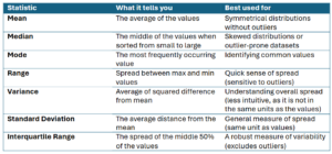
Summary statistics provide a concise overview of a dataset by capturing key aspects such as central tendency, dispersion and distribution. They can help quickly understand data patterns without having to create visualizations.

Example Dataset: 

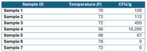
This dataset contains seven samples, each with recorded temperature (in Fahrenheit) and CFU/g (colony-forming units per gram), which measure microbial load, I am not specifying for what, as this is an example.  We will be using the following dataset for our discussion on summary statistics below.  

Measures of central tendency:

Central tendency is concept that describes the center of a variable or multiple variables within a dataset. It represents a single value that summarizes the variable or variables as an indication of where most values fall. The three main measures of central tendency are: 

Mean (Average) 

This is the most common measure of central tendency, we are all very familiar with averages, as these are used. Some examples include and average rating for your favorite restaurant, the average points-per-game of an NBA super star and so on.  

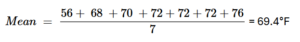
Mathematically, the mean (average) is the sum of all values divided by the number of values. In the example above we can get the mean of the CFU/g column (variable). Where on the denominator we add all the results from each sample and divide it by the number of samples.  

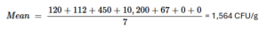
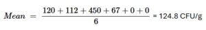
Note: As you can see the average, we got is way higher than most numbers in the column. This is because the mean (average) is very sensitive to extreme values. See above (10,200) is a very large number, if you were to remove this number from the calculation, the new mean would be 124 CFU/g (10-fold lower). Showing that this value is extreme.  

Median  

The median is a little bit less common than the average, but it is used when we want to represent the middle of a distribution. For example, for income data, the median salary is often reported instead of the average because a few very high salaries can make the average misleading 

Mathematically, the median is the middle value when the data is arranged in ascending or descending order. If there is an even number of values, the median is the average of the two middle values.  Let’s calculate the median of the temperature column (variable). 

Note: It is less affected by outliers than the mean. 

Mode (most common value) 

The mode is the frequently occurring value(s) in the dataset. In our Temperature example, we have the following numbers: 56, 68, 70, 72, 72, 72, 76. In this scenario, the mode would be 72, as it repeats itself three times.  

Central tendency when to use which?  

• The mean is best when the data is symmetrically distributed without outliers.  

•  The median is better for skewed distributions or datasets with outliers.  

• The mode is useful for categorical data or identifying the most common occurrence. 

Below you will see the effect of the mean and median on asymmetrical distribution and a skewed distribution.

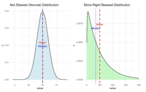
• A normal distribution is symmetrical (mean ≈ median). 

• A right-skewed distribution has a long tail to the right (mean > median). 

• A left-skewed distribution has a long tail to the left (mean < median). 

 

Measures of Variability 

After identifying the center of the data using mean, median and mode, the next critical step is to understand how spread out the data is. This helps answer questions like: 

• Are the values tightly clustered around the average? 

• Is there a lot of variability in the data? 

• Are there any unusually high or low values that might skew the analysis? 

Understanding variability is essential when comparing datasets or interpreting results, especially when making decisions based on consistency or uncertainty. 

The most common measures of variability include: 

Range 

Range is the simplest way to describe the spread. It is calculated as:  

In our Temperature example, our range would be 20°F. 20=76−56. Meaning that the minimum and maximum temperatures are 20°F from each other.  

• A small range suggests that all values are close to each other 

• A larger range could indicate outliers or a wider spread.  

Note: the range is highly sensitive to outliers. Often good to be paired with the interquartile range (IQR).

Interquartile Range (IQR) 

The Interquartile Range (IQR) is a measure of variability that describes the spread of the middle 50% of your data. It’s especially helpful when you’re working with skewed data or datasets with outliers since it focuses on the center of the distribution and excludes extreme values. 

To find the IQR, you first break your sorted dataset into four equal parts (quartiles): 

• Q1 (First Quartile): 25% of the data falls below this value.

• Q2 (Second Quartile): the median, introduced in the central tendency section (50th percentile). 

• Q3 (Third Quartile): 75% of the data falls below this value.

For example, using our temperature data 56, 68, 70, 72, 72, 72, 76.

This means the middle 50% of temperatures fall within a 3°F range. 

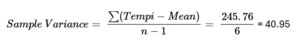
Variance 

Variance measures the average squared difference between each data point and the mean. It gives us an idea of how much the values in a dataset differ from the mean, but because it’s based on squared differences, it’s not in the same units as the original data. For a measure in the units the same units of the data see the SD section.

A high variance means data points are spread out widely; a low variance means they are clustered closely around the mean. 

Step 1: calculate the mean 

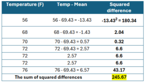
Step 2: calculate the squared difference

 

Standard deviation

Standard deviation is simply the square root of the variance. It’s expressed in the same units as the original data, which makes it more interpretable.

Let’s continue the example above and let’s calculate the standard deviation.

Generally: 

• A small standard deviation means the data points are close to the mean—the values are pretty consistent. 

• A large standard deviation means the data points are more spread out—there’s more variability in the values. 

 

In summary

Summary statistics are simple but powerful tools to start your data analysis and data cleaning. Remember to start with the basics, and then let the data tell its story. In our next post, we will talk about data visualization and their interpretation.