



When we look at data, we tend to start with summary statistics like the mean or the median. They are useful, but they only tell us something about the central tendency of our results, the typical value. They say nothing about how much that value could move if we had sampled on a different day, from a different spot, or with a few more samples. That missing piece is uncertainty, and knowing how confident we are in a number is just as important as the number itself.
Many times, a single average feels like an answer. A confidence interval is the simplest way to put that uncertainty into perspective.
So, What is a Confidence Interval?
Think about the commute example from a few weeks ago. Suppose you ask three neighbors how long it would take you to get to work. One estimates 40 minutes, another estimates 20 minutes, and the third estimates 30 minutes. The average estimated travel time is 30 minutes. Would you bet your 8:00am meeting on that number? Probably not. If you asked 60 neighbors, and it averages 29 minutes, you would feel much better. A confidence interval puts numbers on that feeling; it is a range around your average, built from the data, that expresses how precisely the average has been pinned down. For a mean, NIST describes the interval as the average plus or minus a multiple of the standard error, and notes that the narrower the interval, the more precise the estimate.
To keep this practical, I simulated a water source where we track generic E. coli (on the log10). In this simulated world, the true mean is 1.8 and a standard deviation of 0.7, I know it because I set it. In real life we never get to peek at the truth, which is exactly why intervals matter and are useful.
What Happens When We Add Samples?
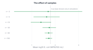
Figure 1 shows six estimates of that same source, using the first 3, 5, 10, 30, 60, and 100 results from one simulated data set. With 3 samples, the average is 1.70 and the interval runs from 0.25 to 3.16, a width of 2.9 log units. With 60 samples, the average is 1.72 and the interval runs from 1.55 to 1.89, a width of 0.34. With 100 samples, the average is 1.73 and the width shrinks to 0.28. So the patter, the sample average gets closer to the true average, and the confidence intervals become narrower.
How is a confidence interval calculated?
Because we are estimating a population mean (the true average of the source) and our sample size is small we can use a t-distribution to calculate the confidence interval, we use the formula:
x̄ ± t* × (s / √n)
Here x̄ is the sample mean, s is the sample standard deviation, and n is the number of samples.
The piece s / √n is called the standard error, and it is what shrinks as n grows.
The multiplier t* comes from the t distribution (these are provided in a table like this one) with n − 1 degrees of freedom, for a 95% interval it is 4.30 when n = 3 and 2.00 when n = 60. When n is large and the data are roughly normal, t* settles close to 1.96 (for a 95% CI), the familiar value from the normal distribution, and the formula becomes x̄ ± 1.96 × s / √n.
Let’s use the first 60 results from our simulated source as a worked example. The mean is 1.72 and the standard deviation is 0.66, so the standard error is 0.66 / √60 = 0.085. Multiplying by t* = 2.00 (which comes from the t table) gives a margin of 0.17, so the 95% interval is 1.72 ± 0.17, or 1.55 to 1.89.
Using the t-distribution is one way to calculate a confidence interval. In this case, the average of roughly bell-shaped data (which I set), so the formula above works well. For proportions, such as a prevalence or the share of samples meeting a limit, other formulas are used, like the Wilson interval, which behave better than the simple formula, especially with small n. A bootstrap interval, which resamples your own data thousands of times, is another option when you do not want to assume the shape of the data. The ideas in this post apply to all of them: more data and less variability give narrower intervals.
What does the “95%” actually mean?
This is the part that trips up even experienced data people.
A 95% interval does not mean there is a 95% chance the true value sits inside this particular interval. It means that if we repeated the sampling many times, about 95% of the intervals we build would capture the truth.
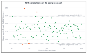
Let’s go back to our water source with n = 10 samples. Because this is a simulation, we know the true mean (1.8) and the standard deviation (0.7), so we can say where the average of 10 samples should land: 1.8 ± 1.96 × 0.7 / √10, which is between 1.37 and 2.23. In other words, if we ran 100 different simulations, we would expect the average to fall outside that range about 5 times. Figure 3 shows exactly that. The dashed lines are the expected range, green dots are averages that fell within it, and orange dots are the ones that did not. Out of the 100 simulations, 95 fell within the range and 5 did not.
Greenland et al. (2016) has nice guide for proper interpreting this information correctly, I recommend it.
So, more sample is better right?
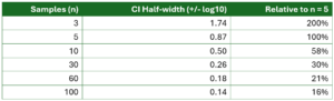
Not always, as we saw above, the width of an interval shrinks with the square root of the sample size. So, the first few samples buy a lot and later ones buy less. Going from 5 to 10 samples cuts the half-width from 0.87 to 0.50. Going from 30 to 100 only moves it from 0.26 to 0.14. Under our equation above, to cut the interval in half, you need roughly four times the data.
Take home messages
- Averages and uncertainty: An average or median only describes the center of the results, and a confidence interval adds how precisely that center is pinned down.
- Sample size: More samples give a narrower interval, with diminishing returns. You need about four times the data to halve it. Meaning that when looking at experiments there is a tradeoff between practicality and value
- What “95%” means: It is a property of the method over many repeats, 95% of the time we would expect the mean to fall within this range. 5% we would expect it not to fall within.